Lecture 4: (de)Normalization & Data Warehousing#
Gittu George, January 16 2025
Todays Agenda#
WHAT is a Data Warehouse?
WHY Data Warehouse?
HOW do we build a data warehouse?
Differences
Wrap up
Learning objectives#
Understanding of data warehouse.
Building a data warehouse.
Connecting our learning from previous classes.
Prerequisites#
Before we talk about data warehousing we need to clearly understand about views;
What are views ?
Why do we want to use views?
Different types of views (and when to use what ?)
How to create views ?
Refresher…
Please check here for more details on views.
If you see in the heading I mentioned about
de-normalization, it is the opposite of normalization. But what is normalization? Please check this refresher to refresh your understanding of normalization or your BAIT 507 notes.
***NOTE:***This will be our last class talking about relational databases.
WHAT is a Data Warehouse?#
A Data Warehouse is a Data Management System
Data Analysts and BI Experts query a front end
Data is ingested in the back-end from multiple sources
A Data Warehouse simplifies data access and analysis.
Its indeed data stored in a database but in a denormalized fashion
It’s generally a process,

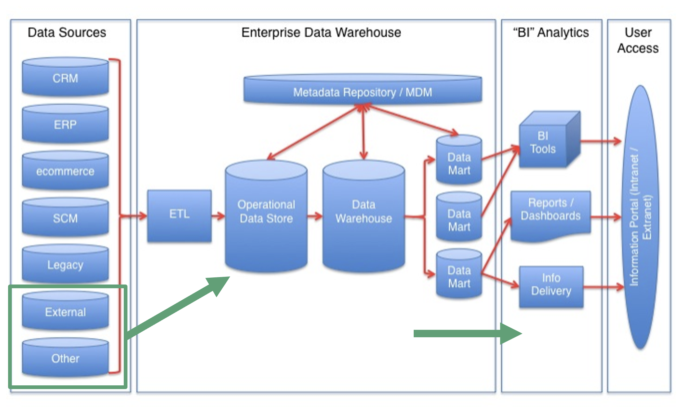
Data moves from data sources to a data warehouse and specialized data marts.
Users access information from the data warehouse/data mart.
Users access data through applications.
When building a data warehouse, we’re taking data from multiple sources and joining it in a comprehensive way to support multiple purposes, from reports and app-based analytics to data mining and machine learning applications.
How do you think a data warehouse may look like?
General structure of Data Warehouse#
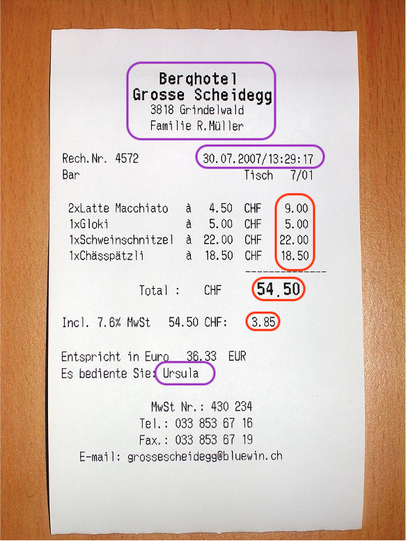
Reciept story#

Image source: wikiMedia
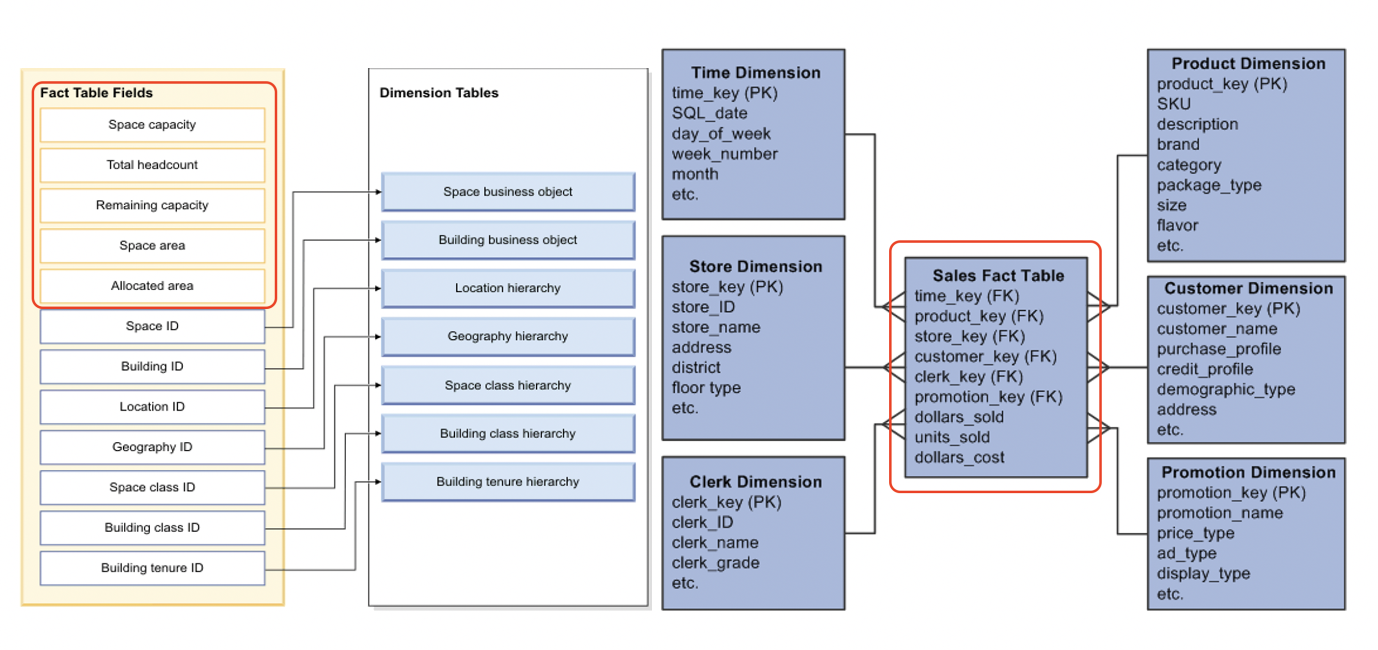
Fact Table: A table that contains the measurements of a business process of interest (in red - above diagram). Dimension Table(s): Tables that provide context for the fact table (in purple - above diagram).
Let’s look at a real world example,

A Data Warehouse results from a process that takes data and transforms it into a “fact table” that a range of users can access. These facts are represented in a manner that is suited to analysis & use by a broad set of users. In addition, it powers up BI Applications like PowerBI or Tableau.
WHY#
Data Can Be Complex
Multiple Sources
Multiple Uses
Multiple Users
Varied Skill Levels
Changing Data & Data Needs
Goals of Data Warehousing & BI#
The Data Warehouse system must:
Make information easily accessible
Present information consistently
Adapt to change
Present information in a timely way
Be secure
Be authoritative & trustworthy
Be accepted by end-users
So How Do We Meet Expectations?#
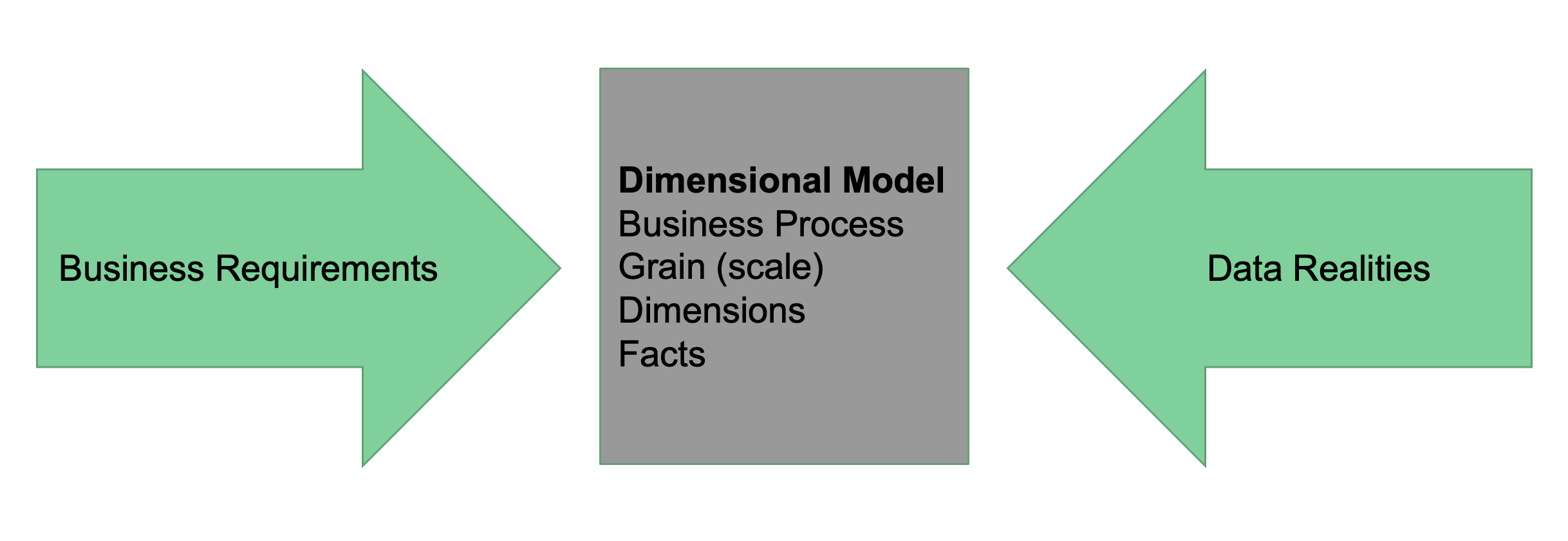
We have this dimensional model influenced by the business requirements & data realities.
The Data Warehouse Design must be collaborative for the expectations to be met. Some parties include;
IT Managers
Executives
BI Analysts
Department Members
App Designers

How Do We Build a Data Warehouse?#
You are already in the process of building an enterprise data warehouse. Here are the steps that you already did;
You identified the data sources
You performed data cleaning and normalization to load the data properly into the database
You are already doing some analysis on the data
Even though you are already doing some joins to get to the analysis, we haven’t properly identified the facts and dimensions for denormalizing the data to one flat table. So let’s go through our Twitter data to see how this process looks like.
in our Twitter data, eg….#
What is the question?
Data we got in hand?
What Facts Do We Need?
What are Facts? What are the Dimensions of those facts?
A Data Warehouse is a type of database, but it conforms to a different data model. It’s focused on a Fact Table with multiple dimensions.
A Data Warehouse is part of a workflow that gets us from raw data (directly from a business process like sales, purchases, quality assessment metrics, real estate holdings, or some other measure) to a dataset easily queried and modeled as part of an analytics team.
Thinking of our Twitter data, we had a central question that asked if daily cashtag volume was positively correlated to stock price changes. So, we took raw tweet data, stock symbol, and price data from multiple sources (Twitter, NYSE, Yahoo! Finance), came up with a data model and undertook data cleaning.
If we’re interested in understanding relationships between the tweets and changes in price, we might want to look at some different analyses. For example:
Sentiment analysis on tweets
Presence of key terms (“sell” or “buy”)
Changes in price
Analysis by individual ticker
Aggregation at different scales (week, month)
If we do that, we would want to work on a single table to undertake our analysis, so we’re assured that there is consistency in our analysis.
Here is the query we might use:
SELECT sy.nasdaqsymbol,
	   sy.securityname,
       cl.tweet,
	   cl.userid,
	   CASE WHEN rp.replyid IS NULL THEN 'FALSE'
	                                ELSE 'TRUE' END AS reply,
	   CASE WHEN rt.retweetid IS NULL THEN 'FALSE'
	                                ELSE 'TRUE' END AS retweet,
	   ROUND(sv.open::numeric,2) AS open,
	   ROUND(sv.close::numeric, 2) AS close,
	   ROUND(sv.close::numeric, 2) - ROUND(sv.open::numeric,2) AS change,
	   date_trunc('day', cl.createdate)::date AS day
FROM          tweets.cashtags AS ct
INNER JOIN tweets.cleantweets AS cl ON cl.tweetid = ct.tweetid
INNER JOIN     tweets.symbols AS sy ON sy.symbolid = ct.symbolid
INNER JOIN tweets.stockvalues AS sv ON sv.symbolid = sy.symbolid AND sv.date = date_trunc('day', cl.createdate)::date
LEFT JOIN      tweets.replies AS rp ON rp.tweetid = cl.tweetid
LEFT JOIN     tweets.retweets AS rt ON rt.tweetid = cl.tweetid;
We’re putting back the columns together and making some decisions about how we treat the data; for example, we’re just adding a boolean (TRUE/FALSE) as to whether something is tweeted or retweeted (using the CASE WHEN statements).
To create the wide table, given that this is essentially a derived table, we’re going to use a MATERIALIZED VIEW. This means that the output is committed to the disk, but it results from a query, so it’s not something we’re going to update directly.
So our call would look something like this:
import pandas as pd
import matplotlib.pyplot as plt
import psycopg2
import json
import urllib.parse

%load_ext sql
%config SqlMagic.displaylimit = 20

with open('credentials.json') as f:
    login = json.load(f)

username = login['user']
password = urllib.parse.quote(login['password'])
host = login['host']
port = login['port']
---------------------------------------------------------------------------
ModuleNotFoundError                       Traceback (most recent call last)
Cell In[1], line 2
      1 import pandas as pd
----> 2 import matplotlib.pyplot as plt
      3 import psycopg2
      4 import json

ModuleNotFoundError: No module named 'matplotlib'
%sql postgresql://{username}:{password}@{host}:{port}/postgres
%%sql
CREATE MATERIALIZED VIEW if not exists tweets.dtwide AS
SELECT sy.nasdaqsymbol,
	   sy.securityname,
       cl.tweet,
	   cl.userid,
	   CASE WHEN rp.replyid IS NULL THEN 'FALSE'
	                                ELSE 'TRUE' END AS reply,
	   CASE WHEN rt.retweetid IS NULL THEN 'FALSE'
	                                ELSE 'TRUE' END AS retweet,
	   ROUND(sv.open::numeric,2) AS open,
	   ROUND(sv.close::numeric, 2) AS close,
	   ROUND(sv.close::numeric, 2) - ROUND(sv.open::numeric,2) AS change,
	   date_trunc('day', cl.createdate)::date AS day
FROM          tweets.cashtags AS ct
INNER JOIN tweets.cleantweets AS cl ON  cl.tweetid = ct.tweetid
INNER JOIN     tweets.symbols AS sy ON sy.symbolid = ct.symbolid
INNER JOIN tweets.stockvalues AS sv ON sv.symbolid = sy.symbolid AND sv.date = date_trunc('day', cl.createdate)::date
LEFT JOIN      tweets.replies AS rp ON  rp.tweetid = cl.tweetid
LEFT JOIN     tweets.retweets AS rt ON  rt.tweetid = cl.tweetid;
 * postgresql://postgres:***@database-1.ccf3srhijxm7.us-east-1.rds.amazonaws.com:5432/postgres
Done.
[]
Look at the “Materialized View” tab in pgAdmin, you’ll see the view there.
I am putting a snapshot of this table on how it looks from pgadmin.


Here are the rows if you check from here using %%sql
%%sql
select * from tweets.dtwide limit 5;
 * postgresql://postgres:***@database-1.ccf3srhijxm7.us-east-1.rds.amazonaws.com:5432/postgres
5 rows affected.
| nasdaqsymbol | securityname | security_ts | tweet | tweet_ts | userid | reply | retweet | open | close | change | day |
|---|---|---|---|---|---|---|---|---|---|---|---|
| A | Agilent Technologies, Inc. Common Stock | 'agilent':1 'common':4 'inc':3 'stock':5 'technologies':2 | @Reforma @lopezobrador_ J$U $A $N Z $E $P $E $D $A ES CUATE DEL P $R $Í $. LA LANA MANDA ?????? | 'a':5,12 'cuate':14 'd':11 'del':15 'e':8,10 'es':13 'j':3 'la':19 'lana':20 'lopezobrador':2 'manda':21 'n':6 'p':9,16 'r':17 'reforma':1 'u':4 'z':7 'í':18 | 842521275411173376 | TRUE | FALSE | 53.97 | 53.92 | -0.05 | 2017-05-18 |
| A | Agilent Technologies, Inc. Common Stock | 'agilent':1 'common':4 'inc':3 'stock':5 'technologies':2 | @Reforma @lopezobrador_ J$U $A $N Z $E $P $E $D $A ES CUATE DEL P $R $Í $. LA LANA MANDA ?????? | 'a':5,12 'cuate':14 'd':11 'del':15 'e':8,10 'es':13 'j':3 'la':19 'lana':20 'lopezobrador':2 'manda':21 'n':6 'p':9,16 'r':17 'reforma':1 'u':4 'z':7 'í':18 | 842521275411173376 | TRUE | FALSE | 53.97 | 53.92 | -0.05 | 2017-05-18 |
| A | Agilent Technologies, Inc. Common Stock | 'agilent':1 'common':4 'inc':3 'stock':5 'technologies':2 | Agilent Technologies Inc $A Shares Bought by Toronto Dominion Bank https://t.co/rPRmDLPkXV | '/rprmdlpkxv':13 'a':4 'agilent':1 'bank':10 'bought':6 'by':7 'dominion':9 'inc':3 'shares':5 't.co':12 't.co/rprmdlpkxv':11 'technologies':2 'toronto':8 | 849417718642159616 | FALSE | FALSE | 53.97 | 53.92 | -0.05 | 2017-05-18 |
| A | Agilent Technologies, Inc. Common Stock | 'agilent':1 'common':4 'inc':3 'stock':5 'technologies':2 | $A received a new alert. Find out why at https://t.co/nZwqReM0tj #stocks #daytrading #trading #mkt #NYSE #NASDAQ #markets 514 | '/nzwqrem0tj':12 '514':20 'a':1,3 'alert':5 'at':9 'daytrading':14 'find':6 'markets':19 'mkt':16 'nasdaq':18 'new':4 'nyse':17 'out':7 'received':2 'stocks':13 't.co':11 't.co/nzwqrem0tj':10 'trading':15 'why':8 | 39546678 | FALSE | FALSE | 53.97 | 53.92 | -0.05 | 2017-05-18 |
| A | Agilent Technologies, Inc. Common Stock | 'agilent':1 'common':4 'inc':3 'stock':5 'technologies':2 | Parametric Portfolio Associates LLC Reduces Stake in Agilent Technologies Inc $A https://t.co/pT9mV2xkRB | '/pt9mv2xkrb':14 'a':11 'agilent':8 'associates':3 'in':7 'inc':10 'llc':4 'parametric':1 'portfolio':2 'reduces':5 'stake':6 't.co':13 't.co/pt9mv2xkrb':12 'technologies':9 | 849417718642159616 | FALSE | FALSE | 53.97 | 53.92 | -0.05 | 2017-05-18 |
It’s a table with three million rows, so we may want to add some indices to the table to speed up our query speed - This is based on the types of questions (queries) that users using this data warehouse will mostly be asking.
For example the only question that I am interested in asking is “The relationship between the number of tweets that are not retweets in a day and the proportional change in stock value”
First, let me drop any indexes that I made previously. (This cell is here just so that the index gets deleted when you run this notebook a second time)
%%sql
drop index if exists tweets.symbolhash_idx;
drop index if exists tweets.nasdaqsymbolhash_idx;
 * postgresql://postgres:***@database-1.ccf3srhijxm7.us-east-1.rds.amazonaws.com:5432/postgres
Done.
Done.
[]
We can directly query our own mini-data warehouse using SQL queries. For example,
The following would give us the relationship between the number of tweets (that are not retweets) in a day and the proportional change in stock value. All of this work then allows us to simplify our workflow and avoid all joins that take lots of time:
%%sql
explain analyze SELECT nasdaqsymbol, ROUND(change / open, 2), COUNT(*) AS tweets
               FROM tweets.dtwide
        WHERE retweet = 'FALSE' AND nasdaqsymbol = 'BABA'
        GROUP BY day, nasdaqsymbol, change, open;
 * postgresql://postgres:***@database-1.ccf3srhijxm7.us-east-1.rds.amazonaws.com:5432/postgres
17 rows affected.
| QUERY PLAN |
|---|
| Finalize GroupAggregate (cost=274785.29..278296.05 rows=26414 width=58) (actual time=14309.616..14312.441 rows=81 loops=1) |
| Group Key: day, change, open |
| -> Gather Merge (cost=274785.29..277671.96 rows=22788 width=26) (actual time=14309.465..14312.336 rows=181 loops=1) |
| Workers Planned: 2 |
| Workers Launched: 2 |
| -> Partial GroupAggregate (cost=273785.27..274041.64 rows=11394 width=26) (actual time=14299.550..14303.634 rows=60 loops=3) |
| Group Key: day, change, open |
| -> Sort (cost=273785.27..273813.76 rows=11394 width=18) (actual time=14299.478..14300.516 rows=8276 loops=3) |
| Sort Key: day, change, open |
| Sort Method: quicksort Memory: 563kB |
| Worker 0: Sort Method: quicksort Memory: 860kB |
| Worker 1: Sort Method: quicksort Memory: 510kB |
| -> Parallel Seq Scan on dtwide (cost=0.00..273017.54 rows=11394 width=18) (actual time=5.644..14290.874 rows=8276 loops=3) |
| Filter: ((retweet = 'FALSE'::text) AND ((nasdaqsymbol)::text = 'BABA'::text)) |
| Rows Removed by Filter: 1171408 |
| Planning Time: 0.631 ms |
| Execution Time: 14312.612 ms |
Wohooo, that was fast, my mini warehouse is helping me, but can we go faster? I see that I am using a condition on retweet and nasdaqsymbol, and I want to execute this query multiple times as it is very important to my business. So I need to think about indexing these 2 columns. Once I have that decision on what kind of indexing makes more sense for those columns.
The nasdaqsymbol and retweet columns could either use a B-TREE index or a HASH index. A HASH index is likely more appropriate if there are few unique symbols and many rows. However, remember that a hash index is only useful for equality. Are we likely to want to analyze stock symbols based on their letter configuration? (e.g., all stocks that start with ‘A’), or is it more likely that we’re just looking at matches?
In our situation, we are interested in exact matches for the stocks we are interested in. In this case, we are interested in nasdaqsymbol to be BABA (I might also be interested in seeing stocks for other companies) and retweets to be FALSE.
%sql CREATE INDEX if not exists nasdaqsymbolhash_idx ON tweets.dtwide USING hash(nasdaqsymbol);
#CREATE INDEX symbolhash_idx ON tweets.dtwide USING hash(retweet);
 * postgresql://postgres:***@database-1.ccf3srhijxm7.us-east-1.rds.amazonaws.com:5432/postgres
Done.
[]
After indexing, let’s look at the time it took to execute our query.
%%sql
explain analyze SELECT nasdaqsymbol, ROUND(change / open, 2), COUNT(*) AS tweets
               FROM tweets.dtwide
        WHERE retweet = 'FALSE' AND nasdaqsymbol = 'BABA'
        GROUP BY day, nasdaqsymbol, change, open;
 * postgresql://postgres:***@database-1.ccf3srhijxm7.us-east-1.rds.amazonaws.com:5432/postgres
12 rows affected.
| QUERY PLAN |
|---|
| HashAggregate (cost=80838.21..81234.09 rows=26392 width=58) (actual time=753.592..753.739 rows=81 loops=1) |
| Group Key: day, change, open |
| Batches: 1 Memory Usage: 793kB |
| -> Bitmap Heap Scan on dtwide (cost=837.87..80564.99 rows=27322 width=18) (actual time=1.965..732.014 rows=24828 loops=1) |
| Recheck Cond: ((nasdaqsymbol)::text = 'BABA'::text) |
| Filter: (retweet = 'FALSE'::text) |
| Rows Removed by Filter: 358 |
| Heap Blocks: exact=2525 |
| -> Bitmap Index Scan on nasdaqsymbolhash_idx (cost=0.00..831.04 rows=27605 width=0) (actual time=0.940..0.940 rows=25186 loops=1) |
| Index Cond: ((nasdaqsymbol)::text = 'BABA'::text) |
| Planning Time: 0.177 ms |
| Execution Time: 753.895 ms |
Excellent! We improved the speed of the query execution.
I plan to use Plotly for visualization, so I am installing it. You might have learned visualization in python using some other packages - please feel free to install those and use those for your assignments (like altair)
! conda install -y plotly
Collecting package metadata (current_repodata.json): done
Solving environment: done


==> WARNING: A newer version of conda exists. <==
  current version: 23.5.0
  latest version: 24.11.2

Please update conda by running

    $ conda update -n base -c conda-forge conda

Or to minimize the number of packages updated during conda update use

     conda install conda=24.11.2


# All requested packages already installed.
%%sql query_output <<

SELECT nasdaqsymbol, ROUND(change / open, 2), COUNT(*) AS tweets
               FROM tweets.dtwide
        WHERE retweet = 'FALSE' AND nasdaqsymbol = 'BABA'
        GROUP BY day, nasdaqsymbol, change, open;
 * postgresql://postgres:***@database-1.ccf3srhijxm7.us-east-1.rds.amazonaws.com:5432/postgres
81 rows affected.
Returning data to local variable query_output
import plotly.express as px
import pandas as pd
fig = px.scatter(query_output,
              x='tweets',
              y='round',
              title='Stock value change by tweet count.',
              hover_name='nasdaqsymbol')
fig.show()
Let me experiment the thread across all the stock tickers;
%%sql query_output <<

SELECT nasdaqsymbol, ROUND(change / open, 2), COUNT(*) AS tweets
               FROM tweets.dtwide
        WHERE retweet = 'FALSE'
        GROUP BY day, nasdaqsymbol, change, open;
 * postgresql://postgres:***@database-1.ccf3srhijxm7.us-east-1.rds.amazonaws.com:5432/postgres
174546 rows affected.
Returning data to local variable query_output
import plotly.express as px
import pandas as pd
fig = px.scatter(query_output,
              x='tweets',
              y='round',
              title='Stock value change by tweet count.',
              hover_name='nasdaqsymbol')
fig.show()
Differences#
DW vs RMDBS#
Database |
Data Warehouse |
|---|---|
Concerned with data security and durability |
Concerned with broad access for analysis |
Highly normalized to ensure referential integrity & reduce update/insertion anomalies. |
Denormalized to ensure ease of access |
Designed to support data ingestion. |
they are only updated by the system |
Data can go in and out |
User data goes out, not in |
ETL vs ELT#
ETL |
ELT |
|---|---|
Extract, Transform and Load |
Extract, Load and Transform |
Data is loaded after performing transformation |
Data first loaded and then transformed |
Mostly used for structured data |
Mostly used for unstructured data |
SQL based databases |
NoSQL based systems |
For building Data Warehouses |
For building data lakes |
OLAP vs OLTP#
OLAP |
OLTP |
|---|---|
Online analytical processing |
Online transactional processing |
Focus on Insert, Update, Delete for databases |
Focuses on extract data for analyzing |
uses the data warehouse |
uses the database |
BI vs DW#
Data warehouse powers up BI. (Business intelligence)
Can you#
Distinguish two different types of views and when to use what?
Define what is data warehousing and why we want it?
How are data warehouses built?
Different terms used in the industry that are related to data warehousing?
Class activity#
Note
Check worksheet 4 in canvas for detailed instructions on activity and submission instructions.
Identify a problem and build a mini data warehouse to answer that question.

